
Interpreting Generate: Parity Plots & Feature Importance
Before trusting or acting on AI‑generated suggestions, inspect the built‑in diagnostics that validate and explain the model’s output.
Overview
Generate surfaces AI‑proposed formulation candidates alongside diagnostics so you can judge predictive quality and model reasoning before acting. Read both the parity and feature‑importance panels together.
Parity plots answer: “Do predictions line up with reality across the range?” Use them to validate accuracy and find blind spots.
Feature importance answers: “What inputs drive the prediction?” Use it to sanity‑check chemistry and detect spurious correlations.
Together: Strong parity + chemically sensible importance ⇒ trustworthy candidates. Any mismatch ⇒ investigate and iterate.
Rule of thumb: don’t ship or scale experiments from Generate until you’ve skimmed both panels and noted at least one actionable insight or caveat.
Interpret this like a pro — quick checklist
Scan parity: any bowing, fanning, or regime where points pull off the diagonal?
Cross‑read importance: do top drivers make chemical sense? Any leaky/operational features?
Decide actions: fill sparse regions (Smart DOE), add descriptors, or remove proxies; then retrain and re‑check.
How to Access the Generate Model Summary
Open the model summary right from your Breakthrough insight. It sits beside the candidate list for quick compare‑and‑decide.
Click your Breakthrough insight to open the Generate results view.
Middle panel: interactive Parity plot. Right panel: open Model summary for the fixed Parity plot and Feature importance.
Use the property dropdown (if available) to switch the target being evaluated (e.g., viscosity, strength).
Hover points/bars for tooltips and filter the candidate list to inspect outliers or top drivers.
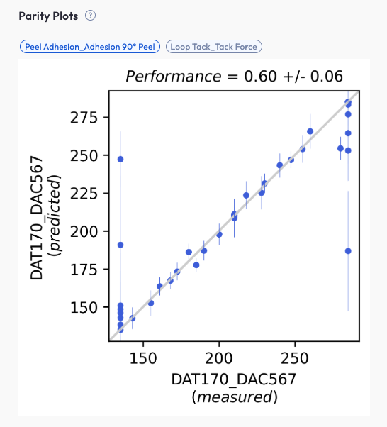
Parity Plots: Validate Predictive Accuracy
A parity plot charts predicted values (Y‑axis) against actual measured values (X‑axis). The diagonal represents perfect predictions.
New: Parity plots were recently updated and are now interactive (hover for point details, zoom/pan).
Legend
Points: individual samples; hover for ID, predicted vs. actual, and error.
Diagonal line: ideal predictions (Predicted = Actual).
Optional bands: tolerance/error bands if enabled.
What good looks like
Points sit close to the diagonal across low → high values.
No big bends or S‑shape.
Error (RMSE/MAE) small for the property scale and enough data points.
Watch‑outs
Underprediction at extremes: sparse data in high or low regimes; model plays it safe.
Clusters or stripes: different batches or units sneaking in.
Wide spread in some ranges: consider a separate model, a simple transform (e.g., log), or a targeted DOE there.
How to act
Filter to outliers and inspect their formulations; confirm measurement quality and units.
Use Smart DOE to target poorly covered regions and rebalance the dataset.
Consider feature engineering (ratios, log transforms) to linearize difficult relationships.
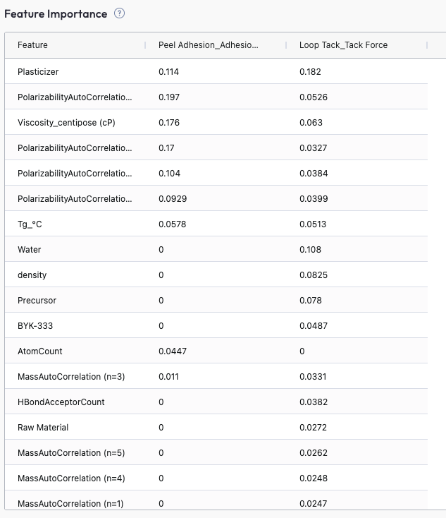
Feature Importance: Reveal What Drives Predictions
Feature importance highlights which inputs most influence the model. Read it as a directional explainability signal—not ground truth.
Feature types you may see
Ingredient amounts: e.g., mass %, phr, mmol ratios for individual raw materials.
Label amounts / tags: grouped totals (e.g., “Solvent content”, “Tag A”) that sum across selected ingredients.
Ingredient properties: measured or catalog attributes (e.g., viscosity of a premix, MW of a polymer grade).
Chemical descriptors: computed features from structure (e.g.,
AtomCount, polarity indices, Hansen parameters, logP, ring count).
Clarification: Terms like AtomCount refer to descriptor‑level features extracted from molecular structure; they’re not lab measurements but computed characteristics.
How to read it
Top drivers should generally align with chemistry (e.g., solvent ratio → viscosity; crosslinker → strength).
Families of related features (e.g., concentrations of A/B/C) may share weight—look at the set, not a single bar.
Compare importance stability across resamples or runs; volatile rankings can indicate data scarcity.
Correlation caveat
If multiple features are highly correlated, they can dilute each other’s individual importance. For example, if you define both Tag A and Tag B to include the same set of ingredients, the model may split the shared signal—so each tag’s displayed importance is roughly half of the combined effect.
Red flags
Missing known factors: suggests limited variance, collinearity hiding effects, or insufficient descriptors.
Operational proxies (e.g., operator name, batch ID) ranking high: risk of leakage and spurious lift.
Single‑feature dominance: may indicate overfitting; check parity and residuals by that feature.
How to act
Add richer descriptors (e.g., molecular descriptors, ratios, interactions) for underrepresented drivers.
Design targeted experiments to break collinearity (vary one driver while holding others steady).
Remove or down‑weight duplicate/correlated tags, or consolidate them into a single, well‑defined tag.
Remove or down‑weight leaky features and retrain.
Example in Practice
Below are concrete formulation‑chemistry scenarios showing how to read parity & feature importance and what to do next.
1) Solventborne Coating — Viscosity Target (700–900 cP) Coatings
Parity: Good in the middle; low predictions at the high end ( ~850 cP).
Drivers: Resin A solids and solvent ratio matter; Thixotrope B looks weak.
Why: Few high‑viscosity runs with B; B moves with Resin A so its effect is hidden.
Try: DOE: 0.5–1.5% B at fixed Resin A; record KU @25 °C and set shear rate. Retrain and check the high end.
2) Waterborne Adhesive — Lap‑Shear Strength Adhesives
Parity: Light S‑shape (a bit high in middle, low at top).
Drivers: Crosslinker:Polyol and dry time high; Tag A and Tag B both show up.
Why: Tag A & Tag B cover the same ingredients → signal is split between them.
Try: Merge tags; run higher crosslinker DOE with controlled cure; log Tg and MW. Retrain.
3) Emulsion — Storage Stability (No Phase Separation @ 40°C, 4 Weeks) Emulsions
Parity: Lots of scatter near the pass/fail boundary.
Drivers: HLB blend, polymer solids, make‑down shear; a calculated aromatic count also shows up.
Why: Aromatic count is a proxy; real effect is HLB × oil polarity.
Try: Add HLB/polarity features; DOE on shear & cooling. Retrain; boundary should look cleaner.
4) Silicone Sealant — Tensile @ 7‑Day Cure Sealants
Parity: Two clusters by supplier.
Drivers: Crosslinker ratio, cure temperature good; supplier looks strong (likely a proxy).
Why: Supplier stands in for moisture/inhibitor differences.
Try: Drop supplier feature; add loss‑on‑drying and inhibitor ppm. Retrain; clusters should merge.
Pattern → Plan: Use parity to spot where the model fails (range, batches, boundary conditions). Use importance to hypothesize why and choose specific variables/regions for the next Smart DOE cycle.
Interactive Parity Plot
GoodBadBiased
Use the Feedback Loop
Diagnose: Read parity for accuracy patterns; scan importance for chemical sense.
Design: Create a Smart DOE batch to fill sparse regions and decouple correlated drivers.
Collect: Run and log results in Albert with clean, standardized units and metadata.
Retrain & Verify: Re‑run Generate; check improved metrics and visuals; note remaining gaps.
Deploy: Push confident candidates to worksheets; document assumptions and watch‑outs.
Cadence: short, iterative cycles beat large one‑off batches. Aim for visible parity/importance improvements each loop.
Why This Matters
Trust: Parity shows whether predictions match reality; spot biases before they reach the bench.
Grounding: Feature importance ties the model to real chemistry and exposes spurious patterns or leakage.
Efficiency: Diagnostics direct where to sample next—maximizing learning per experiment.
Governance: A lightweight, repeatable check before using AI‑guided candidates in R&D decisions.
Questions or feedback? Contact support.